
What is Variation?
Variation is the degree of the difference between an ideal and an actual situation. Variation in a system can result in budget overruns, late order deliveries, long queuing or waiting times, reduced throughput etc.
A simulation is a computer model that mimics the behaviour of a real system by representing operations of a real-world or planned system. The difference between a simulation and an everyday planning model, is that the simulation accounts for variation.
Example
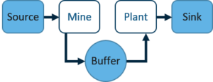
Consider the following example of a Mine feeding into a Plant. If both the Mine and Plant produce throughput at a constant rate of 1 000 tonnes/hour, the output of the system will be 1 000 tonnes/hour.
![]()
In reality, there is some variation in the processing capabilities of these entities. If the Mine is processing at a constant rate of 1 000 tonnes/hour, and the Plant is processing at a varying rate which is sometimes slower than that of the Mine, the total throughput will be slower. In addition, if the Plant is processing at a faster rate than the Mine, the total throughput cannot increase to higher than 1 000 tonnes/hour. Therefore, the throughput will always be lower than the deterministic model due to the presence of variation.
One way in which the effects of variation is often mitigated in real-world scenarios is by placing a buffer between two processes. For demonstration purposes, a buffer is also added to the simulation. By increasing the buffer capacity, overall throughput can be increased. This unfortunately only holds true up to a point whereafter the increased buffer capacity has a negligible effect.
Ideally, the variation can be captured through historical data. This can then be used as distribution inputs for the simulation model to produce accurate results.
Using the Model
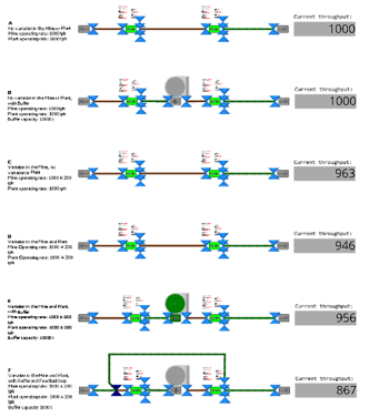
The Model contains six instances (A-F) of the set-up described above with a description of each on the left. The throughput rate is measured on the right of the model.
The deterministic model (A) delivers a throughput rate of 1000 tonnes/hour. This result is the same even when a buffer is added (B). Since the processing rate of the Mine and Plant are matched exactly, the buffer never fills. Instance C shows the Mine operating at a varying rate and in instance D where both the Mine and Plant has variation in processing rate, the throughput is the lowest. By adding a buffer (E) as shown below, the throughput can be improved again as it somewhat mitigates the effect of variation.
Instance F, shown below, demonstrates the effect that a feedback loop can have when a variance is present.
Essentially, a large portion of the material has to pass twice through the Mine and the Plant, thereby compounding the effect of the variation.
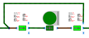
Using the Experimental Model
The Experimental Model depicts a single instance of the set-up as described in instance E. An experimental set-up, under Scenarios, allows for the quick evaluation of the full effect of variation. The larger the variation, the lower the throughput. Varying buffer capacities are also tested in order to demonstrate the relative effect of the buffer. The effect of variance can essentially be mitigated through a buffer. However, the main aim should be to reduce variance as far as possible.
The results of the various scenarios can be visually compared under the Response Results tab. The first seven scenarios demonstrate the effect that variation has on the throughput. The next seven show the effect of an increasing buffer size.